Paper: Not All Water Consumption Is Equal: A Water Stress Weighted Metric for Sustainable Computing

https://dl.acm.org/doi/10.1145/3757892.3757904

Abstract: Water consumption is an increasingly critical dimension of computing sustainability, especially as AI workloads rapidly scale. However, current water impact assessment often overlooks where and when water stress is more severe. To fill in this gap, we present SCARF, the first general framework that evaluates water impact of computing by factoring in both spatial and temporal variations in water stress. SCARF calculates an Adjusted Water Impact (AWI) metric that considers both consumption volume and local water stress over time. Through three case studies on LLM serving, datacenters, and semiconductor fabrication plants, we show the hidden opportunities for reducing water impact by optimizing location and time choices, paving the way for water-sustainable computing. The code is available at https://github.com/jojacola/SCARF.

(See data_centre_water_consumption for an introduction to water consumption by datacentres)

This paper makes the reasonable case that water consumption in different locations and at different times will have a very different impact (or Adjusted Water Impact (AWI)) on local water stress levels. Water usage metrics for eg: datacentres can look small compared to the an entire country, but we must remember that that water consumption is not spread evenly but is located in a small number of communities.

The paper considers scope-1 water consumption (water consumed directly on-site for eg: cooling) and scope-2 (off-site water consumption for electricity generation). The temporal modelling looks at seasonality of water stress, but also projects out into the future using Business-As-Usual (BAU) scenarios and a discount rate to adjust for the the time value of resources.

The authors look at three water consumption cases: LLM inference serving, overall datacentre operation, and semiconductor fabs. All three show significant AWI variation based on geography, but the LLM case is probably the most fleshed out and also includes seasonality results

As the authors note:

The adjusted water impact of deploying LLMs is highly location-sensitive. Same workloads can have orders-of magnitude differences in adjusted water impact depending on where they are served. Even in the same location, seasonal changes can significantly affect adjusted water impact

Notes

• SCARF (Stress-Corrected Assessment of Water Resource Footprint): framework to evaluate water impact of computing by factoring in both spatial and temporal variations in water stress (the ratio of local water demand to supply). Calculates an Adjusted Water Impact (AWI) metric that considers both consumption volume and local water stress over time.
• “Recent studies show that serving 10 to 50 medium length queries from a large language model (LLM) such as GPT-3 can consume 500 mL of water” - but measuring_the_environmental_impact_of_delivering_ai_google_scale estimates 0.26 mL per query, or 100-500x lower.
• “One Google datacenter in Iowa consumed about 3.7 million cubic meters of water in a year” - that’s Council bluffs from https://www.gstatic.com/gumdrop/sustainability/google-2024-environmental-report.pdf which consumes 980.1 million gallons. But that’s many datacentres across two campuses.
• “Intel reported its annual global water consumption of 9.6 million cubic meters.” - that’s tiny, is semiconductor manufacturing really a water issue?
• “focus on Scope 1 water consumption (i.e., water consumed directly on-site, such as in cooling systems) and Scope 2 (i.e., off-site water consumption associated with electricity generation). Scope 3 (i.e., water consumed in upstream supply chain) is not discussed due to the lack of public data”
• Most existing work on water modelling and environmental impact
  • focuses solely on amount of water consumed only, ignoring spatial variability in water stress (1L of water consumed in CentralCalifornia is more impactful than 1L in the Mississippi River Basin)
  • uses static water data, not accounting for how water stress evolves over time due to climate change or long-term resource depletion.
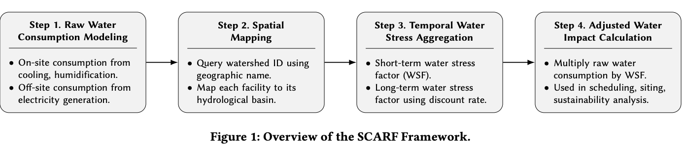
• SCARF process:
  • 
  1. Model water consumption volume, including both on-site (Scope 1) and off-site (Scope 2) consumption.
     • $W_{on}=P\cdot t\cdot {\text{WUE}}_{on}$, where $W_{on}$ is onsite water consumption (in litres), $P$ is the average power draw (in kW), $t$ is the runtime (in hours), and ${\text{WUE}}_{on}$ is onsite water usage effectiveness (in litres/kWh)
     • $W_{off}=P\cdot t\cdot \text{PUE}\cdot {\text{WUE}}_{off}$, where $W_{off}$ is offsite water consumption (in litres), $P$ is the average power draw (in kW), $t$ is the runtime (in hours), ${\text{WUE}}_{off}$ is offsite water usage effectiveness (in litres/kWh), and PUE is Power Usage Effectiveness calculated by dividing the total energy used by the facility by the energy used by its IT equipment
  2. Map each site to its corresponding hydrological basin because water stress varies by watershed, not by country or region.
     • Current and projected water stress levels come from the Aqueduct 4.0 dataset maintained by https://www.wri.org/
  3. Calculate a Water Stress Factor (WSF) using cumulative projections over time
     • A time-weighted aggregation of basin-level water stress values.
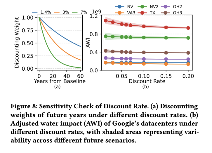
     • To reflect future uncertainty and potential impact, WSF applies a user-defined discount rate 𝛾, following principles from environmental economics. A higher discount rate reduces the weight of future stress; an infinitely large rate ignores future stress entirely.
     • Short-term WSF for short-term analyses, such as evaluating the immediate water stress of computing tasks like LLM serving $WS{F}_b^{\text{short}}=W{S}_{t0,b}$ where $W{S}_{t0,b}$ is water stress at basin $b$ at time 0.
     • Long-term WSF. For long-term facilities like datacenters, which operate for decades, factoring in future water stress provides a more accurate view of sustainability. $WS{F}_b^{\text{long}}={\sum }_{t\in T}{w}_t\cdot W{S}_{t,b}$ where $W{S}_{t,b}$ is water stress at basin $b$ at time $t$, and $w_t$ is computed using a discount rate 𝛾, reflecting the relative importance of future water stress $w_t^{{}^{\prime }}=\frac{1}{(1+\gamma {)}^{t-t_0}},w_t=\frac{w_t^{{}^{\prime }}}{{\sum }_{t^{{}^{\prime }}\in T}{w}_{t^{{}^{\prime }}}^{{}^{\prime }}}$ where $t_0$ is the baseline year, and $T$ is the set of years considered
     • A lower discount rate gives more weight to future water stress, while a higher rate prioritizes near-term impacts.
     • 
     • The choice of discount rate significantly alters datacenter sustainability rankings. A site that is sustainable in the long term (e.g., NV over VA3) may appear less favorable when short-term impacts are prioritized.
  4. Compute the Adjusted Water Impact (AWI) by multiplying total water consumption with the WSF, yielding a unified metric for water sustainability. $\text{AWI}=(W_{\text{on}}+W_{\text{off}})\times WS{F}_b$
• Three case studies, LLM serving, Datacentres, semiconductor fabs.
• Case 1: LLM Serving
  • “LLM serving is flexible and dynamic; cloud providers can shift regions, scale deployments, or update models within months ” - so use short-term water impact.
  • Ran QWEN2.5 (some opensource model) on a single server with a HP100, simulated user queries from open data set.
  • Ran on Azure because WUEs are available (unlike GCP)
  • pynvml and psutil to collect power usage which combined with WUE gives water consumption.
  • 
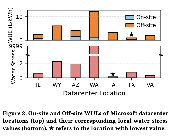
    • Off-site WUE >> on-site
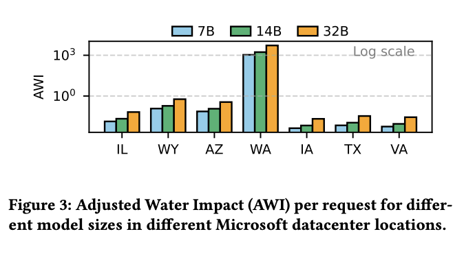
    • Quincy, Washington (WA)—a high-desert area—faces high water stress and less efficient WUE
  • 
    • WA ~1000x worse than IL
  • The adjusted water impact of deploying LLMs is highly location-sensitive. Same workloads can have orders-of magnitude differences in adjusted water impact depending on where they are served.
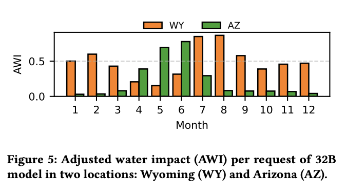
  • AWI also highly variable over the year
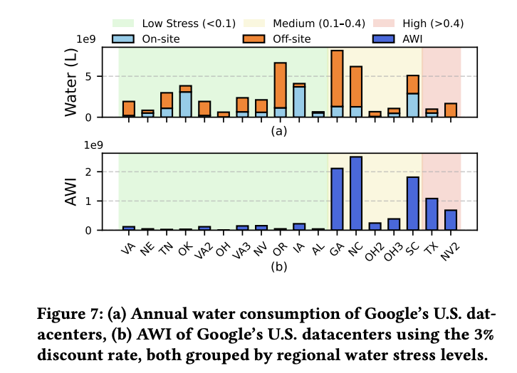
• Case 2: Datacentres
  • evaluate the long-term water impact since datacenters operate for decades
  • Google has best public data for this BUT paper is doing a very rough estimation of total power usage based on based on power capacity of nearby generation sites.
  • Estimates out to 2080, applies a discount rate of 3% and uses the “business as usual” predictions from Aqueduct API
  • 
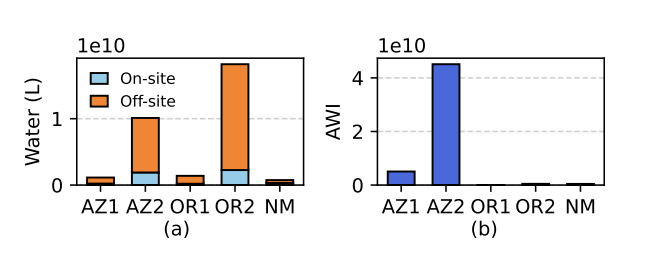
• Case 3: Semiconductor Fab Plants
  • evaluate long-term water impact since these plants operate for decades.
  • Intel has good public data
  • again, BAU and 3% discount rate
  •