Paper: Carbon Aware Computing for Datacenters

https://ieeexplore.ieee.org/stamp/stamp.jsp?tp=&arnumber=9770383

Abstract—The amount of CO2 emitted per kilowatt-hour on an electricity grid varies by time of day and substantially varies by location due to the types of generation. Networked collections of warehouse scale computers, sometimes called Hyperscale Computing, emit more carbon than needed if operated without regard to these variations in carbon intensity. This paper introduces Google’s system for global Carbon-Intelligent Compute Management (CICM) , which actively minimizes electricity-based carbon footprint and power infrastructure costs by delaying temporally flexible workloads. The core component of the system is a suite of analytical pipelines used to gather the next day’s carbon intensity forecasts, train day-ahead demand prediction models, and use risk-aware optimization to generate the next day’s carbon-aware Virtual Capacity Curves (VCCs) for all datacenter clusters across Google’s fleet. VCCs impose hourly limits on resources available to temporally flexible workloads while preserving overall daily capacity, enabling all such workloads to complete within a day with high probability. Data from Google’s in-production operation shows that VCCs effectively limit hourly capacity when the grid’s energy supply mix is carbon intensive and delay the execution of temporally flexible workloads to “greener” times.

This is the rare paper that describes an actual working productionised system. Personal disclosure: I’ve contributed some code to this system as part of my day job. Specifically the pipelines that are used to generate and record the carbon intensity and efficiency day-ahead predictions.

CICM takes advantage of the fact that while the type or size of individual workloads in a cluster are hard to predict, they are predictable in aggregate with a reasonable degree of accuracy when you get to a large enough scale. You make these predictions for inflexible (can’t wait to run) and flexible (can wait up to 1d to run) workloads, combine them with the day-head local grid carbon intensity forecasts, and now you can time-shift your flexible workloads to minimise your daily carbon emissions.

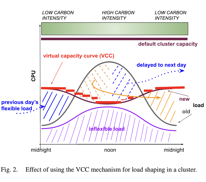
The mechanism to spread out the inflexible workloads is a “virtual capacity curve”, a per-hour artificially lowered compute limit the cluster scheduler must honour while giving precedence to inflexible workloads.

Apart from the predicted flexible and inflexible compute load and carbon intensity forecasts, VCCs are also a function of output of trained models that map compute load to power load, prediction uncertainties, and scheduler SLOs.

Mechanically, CICM is composed of a series of pipelines: carbon fetching, power model generation, and load forecasting which are all inputs to the optimisation pipeline which outputs the VCCs.

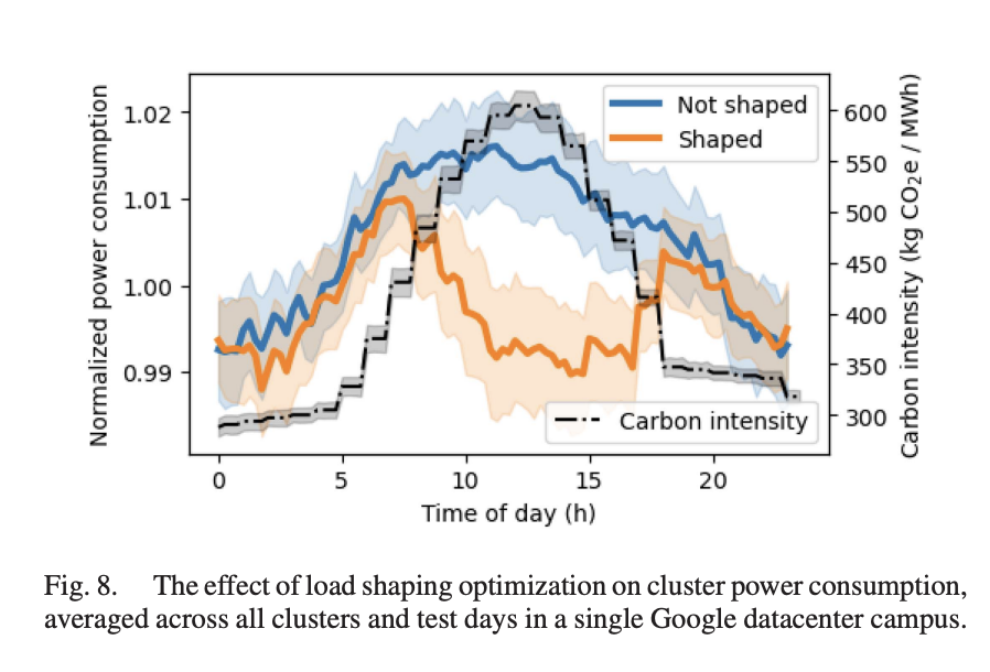
The paper does not provide detailed results across Google’s fleet, but note that “using actual measurements from Google datacenter clusters, we demonstrate a power consumption drop of 1-2% at times with the highest carbon intensity”. If we are generous and assume a 2x factor difference in carbon intensity between high and low hours, that’s 0.5-1% emissions saving which is not exactly earth shattering.

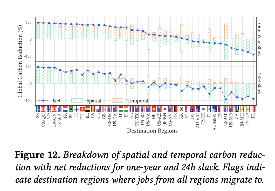
I will note that spatial shifting appears to have much more potential according to On the Limitations of Carbon-Aware Temporal and Spatial Workload Shifting in the Cloud (which I have not read properly), but that also seems like a much harder solution to implement (see Questions below).

Spatiotemporal workload shifting can reduce workloads’ carbon emissions, the practical upper bounds of these carbon reductions are currently limited and far from ideal.” - crucially, temporal carbon intensity varies at most 2x, but spatial up to 43x and spatial is much harder to do.

This paper also points out that

simple scheduling policies often yield most of these reductions, with more sophisticated techniques yielding little additional benefit.

and

The benefit of carbon-aware workload scheduling relative to carbon-agnostic scheduling will decrease as the energy supply becomes greener

Questions

• Batch workloads are easy because they are temporally and spatially flexible. What about serving workloads, is there recent work on Carbon Aware spacial flexibility within latency and legal limits?
• What about ML workloads? These are limited to clusters with specific hardware, the hardware is more heterogenous in its performance and power usage, and CPU is longer the relevant resource, instead it’s some GPU equivalent. Power Modeling for Effective Datacenter Planning and Compute Management which this paper uses does calculate power curves for ML accelerators (and storage devices), but these are not used for carbon aware computing.
• So how do we extend this to spatial flexibility? To minimise emissions over a day, want a set of workload predictions grouped by what clusters can fulfil them (eg: honouring any legal restrictions or HW requirements). Then need create a set of VCC that 1) have enough aggregate capacity to cover all work daily while honoring cluster constraints, 2) with the minimum emissions.

Notes

• This paper is about time-shifting, but there has been followup work on spatial shifting mentioned in https://cloud.google.com/blog/products/infrastructure/using-demand-response-to-reduce-data-center-power-consumption
• Optimising scheduling decisions at the job-level is infeasible for hyperscale clusters with many many jobs.
• System described is in production in Google. Takes advantage of temporal flexibility of a large group of jobs that do not have tight completion deadlines, but only need to finish within 24h. Eg: video encoding, ML training, simulations (Waymo?)
• Challenges
  • Can’t predict what what jobs will run over the course of the next day.
  • Have to meet scheduling/completion SLOs while working within system constraints like compute and power capacity.
  • Need to keep the scheduler complexity low to allow it to deal with high throughput
• While we can’t predict individual workloads, we can do a good job of predicting aggregate workloads and resource requirements a day ahead.
• Virtual Capacity Curves (VCC): per-cluster hourly resource usage limits that serve to shape each cluster resource and power usage profile over the following day. Function of:
  • flexible and inflexible demand predictions
  • prediction uncertainty
  • hourly carbon intensity forecasts
  • explicit business and GHG constraints
  • infrastructure and workload performance expectations (CPU requirements and kW/CPU ?)
  • per-dc power limits provided by utilities
• VCCs calculated a day ahead and pushed to target clusters so they can be used to limit resources per-hour for flexible workloads by delaying scheduling.
• 
• “when delaying the execution of the flexible jobs, their users should be impacted in an unbiased way.”
• VCC computation
  1. Predict next days load
  2. Train models mapping CPU usage to power consumption
  3. Retrieve the next day’s predictions for average carbon intensities on electrical grids where Google’s datacenters reside
  4. Run day-ahead risk-aware, optimization to compute VCCs
  5. Check for flexible workload SLO violations and trigger a feedback mechanism
• The required pipeline are:
  • Carbon fetching pipeline, which reads hourly average carbon intensity forecasts from electricitymaps for grid zones where Google’s datacenters reside (that’s me!)
  • Power models pipeline, which trains statistical models to map CPU usage to power consumption for each power domain (PD) across Google’s datacenter fleet.
    • a PD power consumption can be accurately estimated using only its CPU usage
    • Power model is discussed in https://arxiv.org/pdf/2103.13308 (thing I re-implemented to calculate marginal power consumption based on CPU usage)
    • Power models are developed per PD - so cover a collection of possible heterogenous machines, but the cluster scheduler picks machines randomly - “the resulting CPU usage fractions across PDs within the same cluster varies insignificantly across time”
  • Load forecasting pipeline: predicts inflexible usage hour-by-hour and uncertainty (which is relatively large), but just daily requirements for flexible usage (which is more predictable than an hourly profile and so has low uncertainty).
    • "The effectiveness of the proposed shaping in this paper is mainly due to the high prediction accuracy of the aggregated flexible and inflexible demands"
    • Forecast is done with some EWMA where parameters are chosen such “out-of-sample Mean Absolute Percent Error (MAPE) is minimized”
    • Predict week-ahead, then adjust based on divergence of yesterday’s prediction from previous week-ahead forecast. Adjustment parameters calculated via linear regression to “minimize out-of-sample MAPE.”
  • Optimisation pipeline which takes the above outputs, infrastructure and application SLO constraints, contractual and resource capacity limits, and outputs VCCs that optimise to minimise emissions AND peak power usage (through minimising peak CPU usage, which reduces risk of demand for future infrastructure builds required to support its workload)
  • SLO violation detection pipeline: flags when a cluster’s daily flexible demand is not met. If this happens repeatedly, load shaping is turned off to give forecasting a chance to catch up.
  • Carbon intensity forecasting pipeline: using electricity maps
• Sum under the VCC curve must be at least 97% of the sum of the flexible and inflexible capacity reservations (not usage) of the day.
• Impact
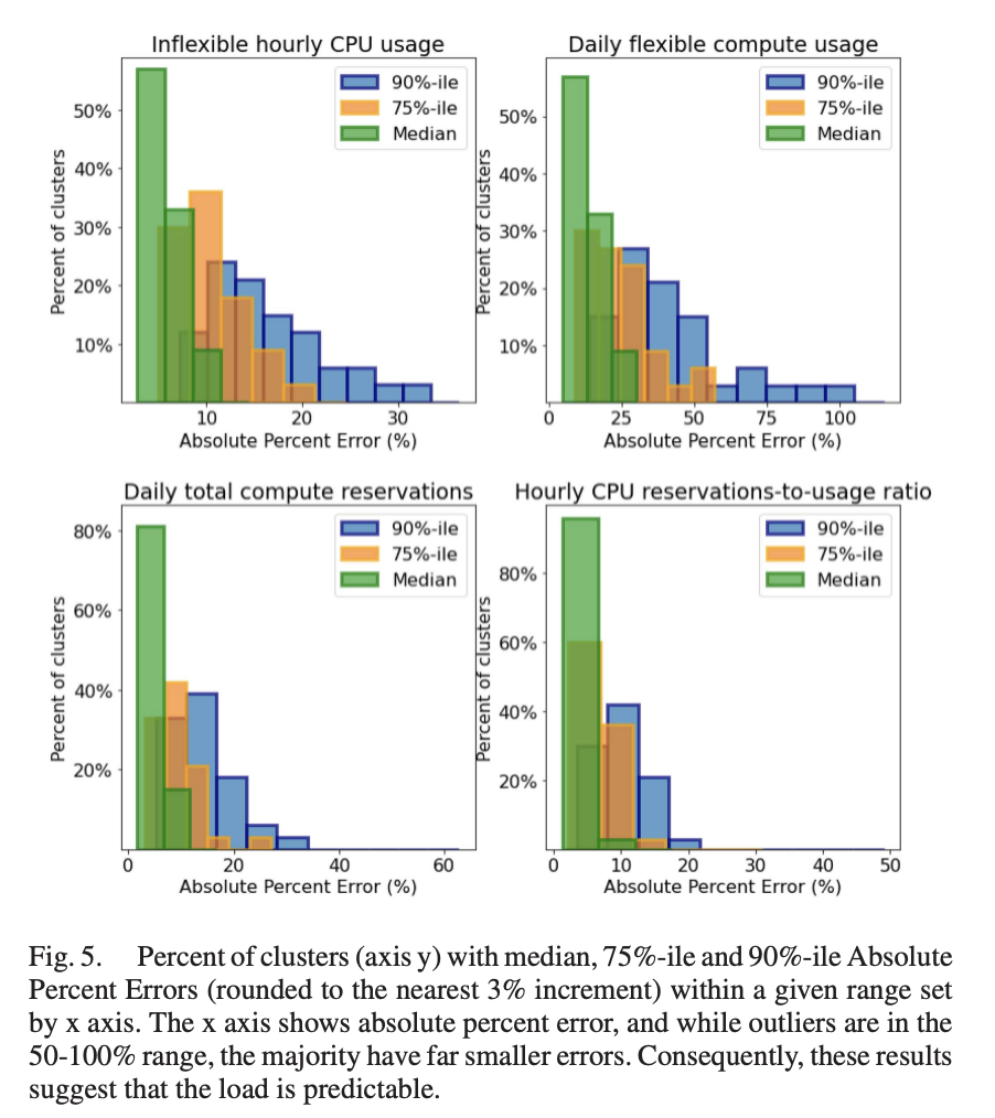
  • Prediction errors relatively low , except for flexible usage since that is often more volatile, especially in smaller clusters:
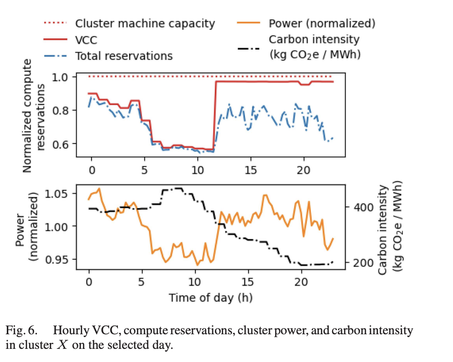
  • Example - note that the VCC could have shifted more load to later in the day when emissions were lower, but the forecast uncertainty limits how tightly we can run things:
  • Normalized power curves, averaged across all datacenter clusters in a campus, on randomly treated (optimized) and non-treated (not optimized) days for two months beginning February 12th 2021: