Distributed Energy Resources - Lecture 4: Linear Dynamical Systems

Other notes in this series from Kevin Kircher’s Distributed Energy Resources class are here.

Summary

This lecture builds on the scalar and vector linear ODEs in DER course - 3 to model Linear Dynamical Systems: “models that describe how a system changes over time, where the relationships between its variables are all linear”, then finishes up with a fun little climate model as practical example.

• A continuous-time linear dynamical system (LDS)
  $\frac{dx(t)}{dt}=A(t)x(t)+B(t)u(t)+w(t)$
  • $t\in R$ denotes time
  • $x(t)\in R^{n_x}$ is the state
  • $u(t)\in R^{n_u}$ is the action or control
  • $w(t)\in R^{n_x}$ is the disturbance
  • $A(t)\in R^{n_x\times n_x}$ is the dynamics matrix
  • $B(t)\in R^{n_x\times n_u}$ is the action matrix or control matrix
• We can use the matrix equivalent of Taylor’s theorem to linearise non-linear
• If we discretise:
  • Consider the continuous-time LDS
    $\frac{dx(t)}{dt}=\tilde{A}(t)x(t)+\tilde{B}(t)u(t)+\tilde{w}(t)$
    with piecewise constant $\tilde{A},\tilde{B},u,\tilde{w}$
  • The equivalent discrete-time LDS is:
    $x(k+1)=A(k)x(k)+B(k)u(k)+w(k)$
    where $.(k)$ denotes $.(t_k)$
    $A(k)=e^{(t_{k+1}-t_k)\tilde{A}(t_k)}$
  • If the dynamics matrix $\tilde{A}(t_k)$ is invertible
    $B(k)=(A(k)-I)\tilde{A}(t_k{)}^{-1}\tilde{B}(t_k)$
    $w(k)=(A(k)-I)\tilde{A}(t_k{)}^{-1}\tilde{w}(t_k)$

Then the fun part: a simple climate model 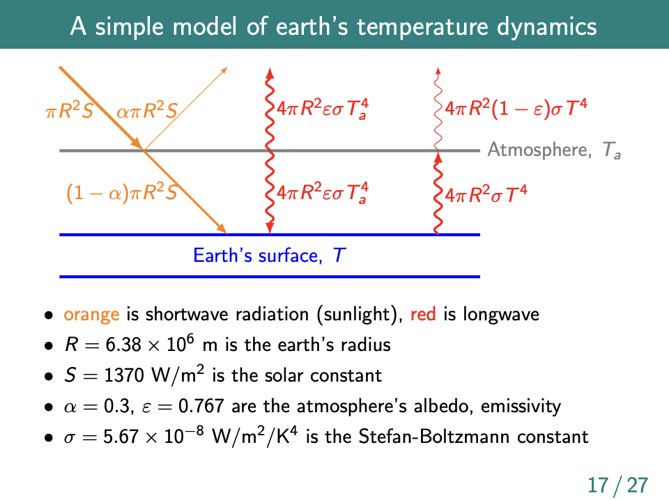Then we do some neat power-balance calculations and end up with

1. Steady state global average surface temperature: $T=\sqrt[4]{\frac{(1-\alpha )S}{4\sigma (1-\epsilon /2)}}$
2. Rate of change: $\frac{dT(t)}{dt}=\frac{\pi R^2}{C}[(1-\alpha (t))S-4\sigma (1-\epsilon (t)/2)T(t{)}^4]$

If we plug in historical temperature and ε values then we get reasonably close numbers! See the lecture notes for details.

Notes

Homework

Some simple Python implementation of the above earth climate model. Non-linear and linearised. The hard part was figuring out what the exercise required.

---

• A continuous-time linear dynamical system (LDS)
  $\frac{dx(t)}{dt}=A(t)x(t)+B(t)u(t)+w(t)$

  • $t\in R$ denotes time
  • $x(t)\in R^{n_x}$ is the state
  • $u(t)\in R^{n_u}$ is the action or control
  • $w(t)\in R^{n_x}$ is the disturbance
  • $A(t)\in R^{n_x\times n_x}$ is the dynamics matrix
  • $B(t)\in R^{n_x\times n_u}$ is the action matrix or control matrix

• A continuous-time LDS with imperfect observations
  $\frac{dx(t)}{dt}=A(t)x(t)+B(t)u(t)+w(t)$
  $y(t)=C(t)x(t)+D(t)u(t)+v(t)$

• $y(t)\in R^{n_y}$ is the observation or output

• $v(t)\in R^{n_y}$ is the noise

• $C(t)\in R^{n_y\times n_x}$ is the observation matrix

• $D(t)\in R^{n_y\times n_u}$ is the feedthrough matrix

• Common simplifications

  • time-invariant: $A$, $B$, $C$, and $D$ are independent of $t$
  • single-input, single-output: $nu=ny=1$
  • no feedthrough: $D(t)=0$ for all $t$
  • perfectly observed: $y(t)=x(t)$
  • deterministic: $w(t)=0$ and $v(t)=0$ for all $t$

• Why do we care about linear things when reality is typically non-linear? Linearity helps with tractability. Can often represent non-linear systems pretty well with linear ones.

• For scalars-valued functions, we can linearise with Taylor’s theorem: a mathematical tool that allows us to approximate a function by an infinite sum of terms, where each term is derived from the function’s derivatives at a single point

  • The simplified version is:
    suppose nonlinear $f:R\to R$ is differentiable at $\hat{x}\in R$
    if $x$ is near $\hat{x}$, then $f(x)\approx f(\hat{x})+f^{\prime }(\hat{x})(x-\hat{x})$
  • The full version: $f(x)={\sum }_{n=0}^{\inf }\frac{f^{(n)}(\hat{x})}{n!}(x-\hat{x}{)}^n$

• Similarly, can linearise vector-valued functions of vectors with:
  suppose nonlinear $f:R^n\to R^m$ is differentiable at $\hat{x}\in R^n$
  if $x$ is near $\hat{x}$, then $f(x)\approx f(\hat{x})+D_f(\hat{x})(x-\hat{x})$
  where $D_f(\hat{x})=\left[\begin{array}{ccc}\frac{\delta f_1}{\delta x_1}{|}_{\hat{x}}& \dots & \frac{\delta f_1}{\delta x_n}{|}_{\hat{x}}\\ ⋮& & ⋮\\ \frac{\delta f_m}{\delta x_1}{|}_{\hat{x}}& \dots & \frac{\delta f_m}{\delta x_n}{|}_{\hat{x}}\end{array}\right]\in R^{(m\times n)}$
  this is the derivate matrix or Jacobian matrix of $f$ at $\hat{x}$

• A continuous-time non-linear dynamical system (LDS)
  $\frac{dx(t)}{dt}=f(x(t),u(t),w(t)$ with dynamics function $f:R^{n_x}\times R^{n_u}\times R^{n_w}\Rightarrow R^{n_x}$
  <skipped derivation> $\frac{d{\delta }_x(t)}{dt}\approx A(t){\delta }_x(t)+B(t){\delta }_u(t)+G(t){\delta }_w(t)$
  where
  ${\delta }_x(t)=x(t)-\hat{x}(t),{\delta }_u(t)=u(t)-\hat{u}(t),{\delta }_w(t)=w(t)-\hat{w}(t)$
  and
  $A_{ij(t)}=\frac{\delta f_i}{\delta x_j}{|}_{\hat{x}(t),\hat{u}(t),\hat{w}(t)}$
  $B_{ij(t)}=\frac{\delta f_i}{\delta u_j}{|}_{\hat{x}(t),\hat{u}(t),\hat{w}(t)}$
  $G_{ij(t)}=\frac{\delta f_i}{\delta w_j}{|}_{\hat{x}(t),\hat{u}(t),\hat{w}(t)}$

• For discretised time

  • Perfectly observed LDS $\frac{dx(t)}{dt}=A(t)x(t)+B(t)u(t)+w(t)$
  • Suppose $A$ is piecewise constant:
    $t_k\le t<t_{k+1}\Rightarrow A(t)=A(t_k)$
  • Then
    $x(t_{k+1})=e^{(t_{k+1}-t_k)A(t_k)}x(t_k)+e^{t_{k+1}A(t_k)}{\int }_{t_k}^{t_{k+1}}{e}^{-\tau A(t_k)}(B(\tau )u(\tau )+w(\tau ))d\tau$
  • This is just the ODE IVP solution with $t^{init}=t_k,t=t_{k+1}$ and $b(t)=B(t)u(t)+w(t)$

• Now assume everything except $x$ is piecewise constant:
  $t_k\le t<t_{k+1}\Rightarrow \{\begin{array}{l}A(t)=A(t_k),B(t)=B(t_k)\\ u(t)=u(t_k),w(t)=w(t_k)\end{array}$
  then
  $x(t_{k+1})=e^{(t_{k+1}-t_k)A(t_k)}x(t_k)+e^{t_{k+1}A(t_k)}{\int }_{t_k}^{t_{k+1}}{e}^{-\tau A(t_k)}d\tau (B(t_k)u(t_k)+w(t_k))$
  If $A(t_k)$ is invertible, then
  $e^{t_{k+1}A(t_k)}{\int }_{t_k}^{t_{k+1}}{e}^{-\tau A(t_k)}d\tau =(e^{(t_{k+1}-t_k)A(t_k)}-I)A(t_k{)}^{-1}$

• Summary for discretising LDS:

  • consider the continuous-time LDS
    $\frac{dx(t)}{dt}=\tilde{A}(t)x(t)+\tilde{B}(t)u(t)+\tilde{w}(t)$
    with piecewise constant $\tilde{A},\tilde{B},u,\tilde{w}$
  • The equivalent discrete-time LDS is:
    $x(k+1)=A(k)x(k)+B(k)u(k)+w(k)$
    where $.(k)$ denotes $.(t_k)$
    $A(k)=e^{(t_{k+1}-t_k)\tilde{A}(t_k)}$
    $B(k)=e^{t_{k+1}\tilde{A}(tk)}{\int }_{t_k}^{t_{k+1}}{e}^{-\tau \tilde{A}}d\tau \tilde{B}(t_k)$
    $w(k)=e^{t_{k+1}\tilde{A}(tk)}{\int }_{t_k}^{t_{k+1}}{e}^{-\tau \tilde{A}}d\tau \tilde{w}(t_k)$
  • if the dynamics matrix $\tilde{A}(t_k)$ is invertible
    $B(k)=(A(k)-I)\tilde{A}(t_k{)}^{-1}\tilde{B}(t_k)$
    $w(k)=(A(k)-I)\tilde{A}(t_k{)}^{-1}\tilde{w}(t_k)$
    • There is no general analytical formula for discretising
      $\frac{dx(t)}{dt}=f(x(t),u(t),w(t))$
      with an arbitrary nonlinear dynamics function $f$, but numerical ODE solvers can do the trick